Ace Your Coding Interview by Understanding Big O Notation — and Write Faster Code
The world’s top tech firms test candidates’ knowledge of algorithms and how fast these algorithms run. That’s where Big O Notation comes…

Published on
Mar 2, 2019
Read time
17 min read
Introduction
The world’s top tech firms test candidates’ knowledge of algorithms and how fast these algorithms run. That’s where Big O Notation comes in. This article explains what it is, and provides practical examples of real world algorithms and their Big O Classification.
Understanding how fast your algorithms are going to run is a crucial skill in coding. For smaller data sets, this might not cause too many headaches, but on systems with a large amount of users, data, and more, the difference could be staggering.
While knowledge of Big O Notation is mostly only relevant to the interview process of larger tech firms, it is still well worth knowing how to make your algorithms as fast as possible. Understanding how to write more efficient algorithms and why they’re more efficient is helpful at every level!
Why Efficiency Matters

Image Credit: Inc.
Before going into Big O Notation, I’ll explain why it’s important with a silly example. Let’s say you’ve got 10 emails, and one of those emails contains a phone number you need. You’re not allowed to use the search bar. How do you find the phone number?
Well, it’s only 10 emails, so you probably just open each email one-by-one, scan over it, and open the next email. You keep going until you find the phone-number and — at most — you will have checked 10 emails. That’s no trouble. It’ll only take a minute or two.
Now imagine you have 1.8 billion emails, and you still need that one phone number. Faced with this scale, you would never imagine going through each email. Even if you could check 1 email every second and never sleep, it would still take over 57 years to find the phone number you need!
This example is very silly. If you were so unfortunate as to have 1.8 billion emails, you’d definitely use the search bar (and might I recommend some mass unsubscription software)! But the example demonstrates clearly that a process which works fine on a small scale is completely impractical on a very large scale.
I chose the number 1.8 billion because, in January 2018, that was the estimated number of active websites on the internet, and so that’s roughly the number of websites that search engines like Google need to store data about. It’s crucial, therefore, that services like Google Search make use of the most optimal algorithms in order to deal with all that data.
What is Big O Notation?

At its most basic level, Big O Notation provides us with a quick way to assess the speed — or, more properly, the performance — of an algorithm. It measures how quickly the run-time grows relative to the input, as the input increases.
For many algorithms, it is possible to work how efficient they are out at a glance, and express this using Big O Notation. That’s why many of the world’s top programming companies test this knowledge in interview.
A highly efficient algorithm like Binary Search might have a performance of O(logN), while a horrendously inefficient algorithm like Bogosort might have a performance of O(log(N!)).
If this all looks unfamiliar, don’t worry. I’ll introduce the necessary details one-by-one. This article is intended for beginners, but it also goes a deeper than any other article for beginners that I have encountered. That’s because, in this article, we’ll not only cover the theory of Big O Notation, but we’ll also look at several well-known searching/sorting algorithms in context of Big O Notation, and what the code for those algorithms might look like.
Prerequisites

Image Credit: Wharton University
The example code is written in JavaScript, so you’ll get the most out of this article if you have some understanding of JavaScript. I’m also going to assume at least basic knowledge of arrays, functions and loops.
O(1)
This represents an algorithm whose run-time is fixed. No matter the amount of data you feed in, the algorithm will always take the same amount of time.
In the following example, we pass an array to a function. It doesn’t matter whether the array has 1 entry or 1,000 — it will always take the same amount of time, because it’s simply returning the very first value.
We call that O(1), and any function that spits out one value — regardless of the input size — can be described as having a performance of O(1).
function constantFn(array) {
  return array[0];
}

O(N) — Linear Time
This is the equivalent of going through all your emails by hand. As the length of the array increases, the amount of processing required increases at the same rate.
In this function, every item in an array is printed straight to the console. As the size of the array increases, the number of times console.log() is called increases by exactly the same amount.
function linearFn(array) {
  for (let i = 0; i  array.length; i++) {
    console.log(array[i]);
  }
}
Note that Big O Notation is based on the maximum possible iterations. Because of that, the following function still has an algorithmic efficiency of O(N), even though the function could finish early; that’s why some people see it as a measure of the “worst case scenario”.
function findTheMeaningOfLife(array) {
  for (let i = 0; i < array.length; i++) {
    if (array[i] === 42) {
      return i;
    }
  }
}
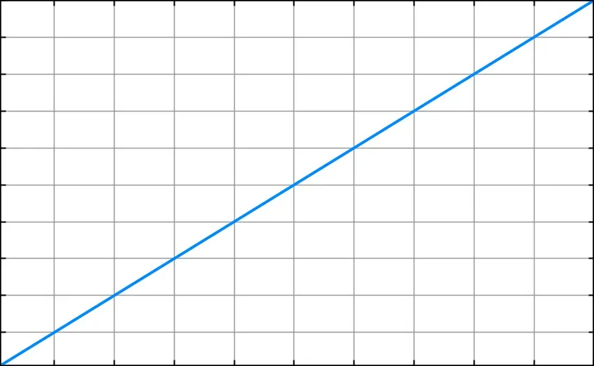
Here’s what this looks like on a line graph, where the x axis represents the amount of data and the y axis represents the run-time.
Note: The bottom-left corner of this graph— and for all the graphs from now on — represents x = 1 and y = 1.
O(N²) — Quadratic Time
An algorithm with an efficiency of O(N²) increases at twice the relative rateof O(N). I’ll demonstrate using console.log.
Let’s say we have an array of three numbers: array = [1, 2, 3].
If we pass that to the function logArray() above, then it will simply print out the numbers 1, 2 and 3.
But what about this function?
function quadraticFn(array) {
  for (let i = 0; i < array.length; i++) {
    for (let j = 0; j < array.length; j++) {
      console.log(array[j]);
    }
  }
}
This will print 1 2 3 1 2 3 1 2 3 to the console.
That’s 9 numbers, compared to the 3 printed by logArray. And so it follows that 3² = 9, and this function has a performance of O(N²).
Here’s another example of an O(N²) function, which return true if adding any two numbers in the array yields 42. As above, it could return early, but we assume it will take the maximum amount of time.
function isSum42(array) {
  for (let i = 0; i  array.length; i++) {
    for (let j = 0; j < array.length; j++) {
      if (array[i] + array[j] === 42) {
        console.log('Found the meaning of life!');
        return true;
      }
    }
  }
}
Bubble Sort
Now for our first example of a real-world sorting algorithm, the Bubble Sort. This sorts an array of values, and its performance can be described as O(N²). First, I’ll explain how the algorithm works. Then, we’ll see what it might look like in JavaScript.
Source: Wikipedia
Let’s start with an unsorted array with values [6, 5, 3, 1, 8, 7, 2, 4].
The Bubble Sort works by comparing each pair of adjacent values, one-by-one. In each pair, if the second number is bigger, the numbers stay where they are. But if the second number is smaller, they swap places.
The first pass
- First the algorithm will compare
6and5. As5is smaller, it move one place back, yielding:[5, 6, 3, 1, 8, 7, 2, 4] - Next, we compare
6and3. As3is smaller, it will move a step back, yielding:[5, 3, 6, 1, 8, 7, 2, 4]. - The pattern continues 7 times until the algorithm reaches the final item of the array, and we’re left with an array like this:
[5, 3, 1, 6, 7, 2, 4, 8].
How many passes do we need?
- After the first pass, our array isn’t sorted, but it’s going in the right direction. We need to keep going, using as many passes as it takes until no numbers need to be swapped.
- The algorithm runs a second pass, starting at the beginning. When it is done, the array is now:
[3, 1, 5, 6, 2, 4, 7, 8] - The third pass yields:
[1, 3, 5, 2, 4, 6, 7, 8] - The fourth pass yields:
[1, 3, 2, 4, 5, 6, 7, 8] - The fifth pass yields:
[1, 2, 3, 4, 5, 6, 7, 8] - If we try to run a sixth pass, none of the items would change order. We know, therefore, that the items are sorted. In this case, it took 5 passes.
Why the Bubble Sort has a performance of O(N²)
The reason the bubble sort’s performance is O(N²) becomes clear when you look at a function that uses this method.
Here is a simple implementation, which runs the maximum number of passes that might be needed.
(A more sophisticated bubble sort would prevent the algorithm from continuing once no swaps where made — but to keep things simple, I have left this out.)
function bubbleSort(array) {
  let length = array.length;

  // This loop handles the passes
  for (let i = 0; i < length; i++) {

    // This loop handles the swapping during a single pass
    for (let j = 0; j < (length - i - 1); j++) {
      if (array[j]  array[j + 1]) {
        let tmp = array[j];

        array[j] = array[j + 1];
        array[j + 1] = tmp;
      }
    }
  }

  return array;
}
As you can see, there are two for loops, and the second is nested in the first. That is a classic sign that we are dealing with O(N²). And that’s our first real-world performance analysis of an algorithm using Big O Notation!
O(N³), O(N⁴) — Cubic Time, Quartic Time, and so on
If two nested loops gives us O(N²), it follows that three nested loops gives us O(N³), four nested loops gives us O(N⁴), and so on.
Let’s return to our simple array [1, 2, 3], and pass it to the following with a performance of O(N³):
function cubicFn(array) {
  for (let i = 0; i  array.length; i++) {
    for (let j = 0; j < array.length; j++) {
      for (let k = 0; k < array.length; k++) {
        console.log(array[k]);
      }
    }
  }
}
The output is 27 (= 3³) numbers — which is exactly what we’d expect, given our input N has a value of 3.
1 2 3 1 2 3 1 2 3 1 2 3 1 2 3 1 2 3 1 2 3 1 2 3 1 2 3
If we added yet another loop, we’d get a function like this:
function quarticFn(array) {
  for (let i = 0; i < array.length; i++) {
    for (let j = 0; j < array.length; j++) {
      for (let k = 0; k < array.length; k++) {
        for (let l = 0; l < array.length; l++) {
          console.log(l);
        }
      }
    }
  }
}
This O(N⁴) function yields 81 (= 3⁴) numbers, exactly as we would expect:
1 2 3 1 2 3 1 2 3 1 2 3 1 2 3 1 2 3 1 2 3 1 2 3 1 2 3 1 2 3 1 2 3 1 2 3 1 2 3 1 2 3 1 2 3 1 2 3 1 2 3 1 2 3 1 2 3 1 2 3 1 2 3 1 2 3 1 2 3 1 2 3 1 2 3 1 2 3 1 2 3
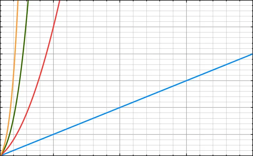
And so the pattern continues. You can see in the graph below that as the powers increase, the run-time of each algorithm increases drastically at scale.
Why We Often Ignore Multiples
Let’s say for every item we put into our function, it processes the data twice over. For example, we could have a function like this:
function countUpThenDown(array) {
  for (let i = 0; i < array.length; i++) {
    console.log(i);
  };

  for (let i = array.length; i  0; i--) {
    console.log(i);
  };
}
We could call that O(2N). And, if we added another for loop to the sequence, so that it processed the data a third time we could call it O(3N).
At small scales, the difference is very important. But Big O Notation is concerned with how an algorithm functions at a very high scale. For that reason, we tend to ignore multiples.
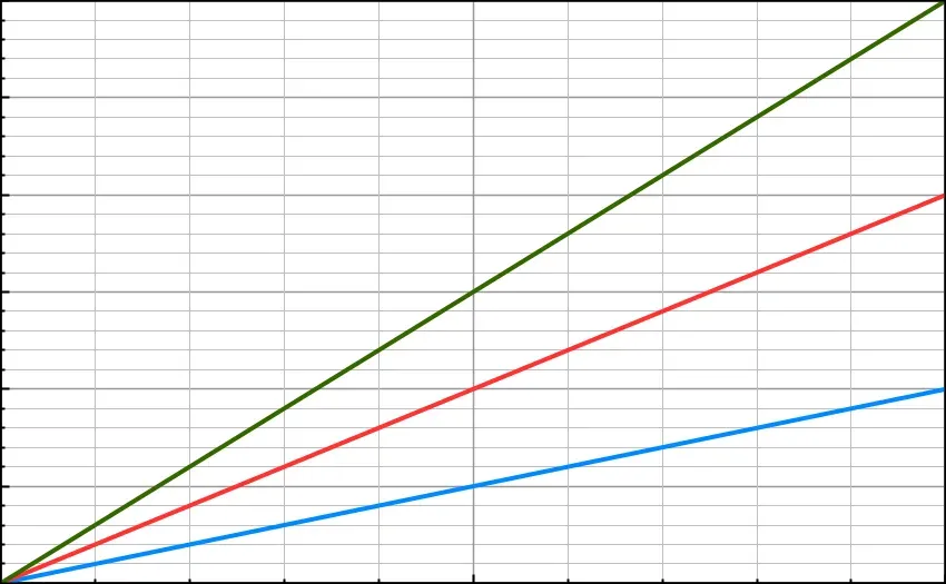
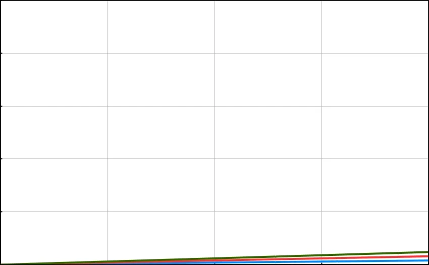
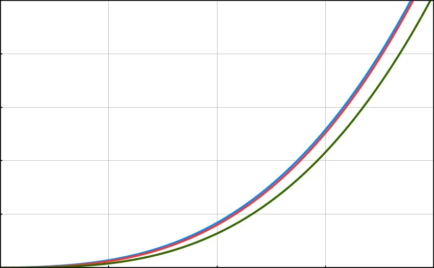
Blue: O(N) · Red: O(2N) · Green: O(3N). The image on the right is zoomed-out, to illustrate how the differences are much less significant on a larger scale.
The graph above on the left shows the difference between O(N) and O(2N) at a small scale. The graph above on the right demonstrates that this difference becomes insignificant at a much larger scale.
The same goes for multiples of powers, such as O(2N²). The graph below includes O(N), O(2N), O(N²) and O(2N²):
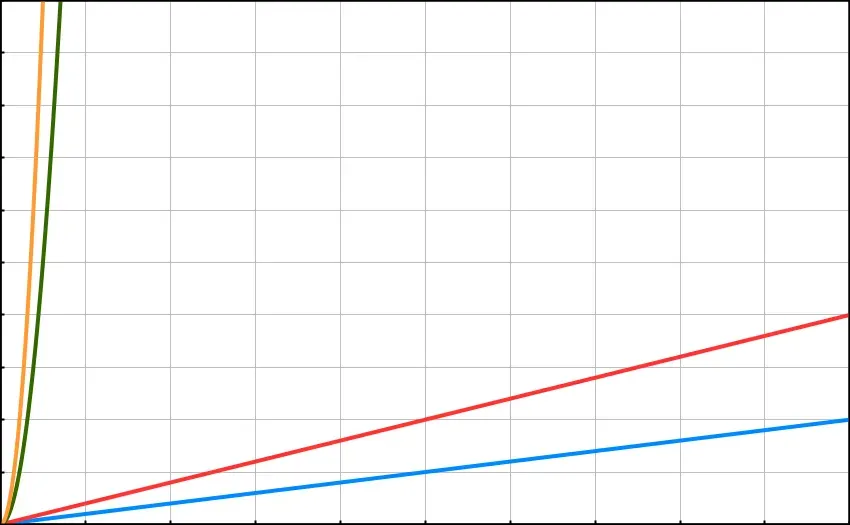
On this scale, there is some difference between O(N) and O(2N), but it is relatively little. As for O(N²) and O(2N²) — they are even closer together.
In general, we consider the difference between linear O(N) and quadratic O(N²) — and so on — to be much more significant than the difference between multiples of the same type. So, in most cases, you can safely ignore multiples.
Why We Often Ignore All But the Biggest Power
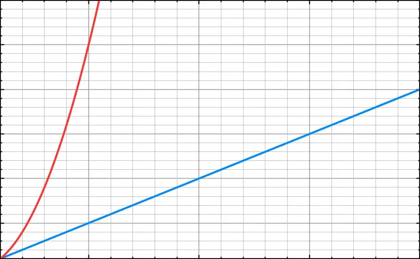
For the exact same reason, you’ll rarely see a function’s efficiency described as O(N² + N). In fact, the difference between O(N² + N) and O(N²) increases — by the order of N — as the scale increases. Nevertheless, in most cases we shorten O(N² + N) to simply O(N²) because it is this which commands the scaling of the algorithm.
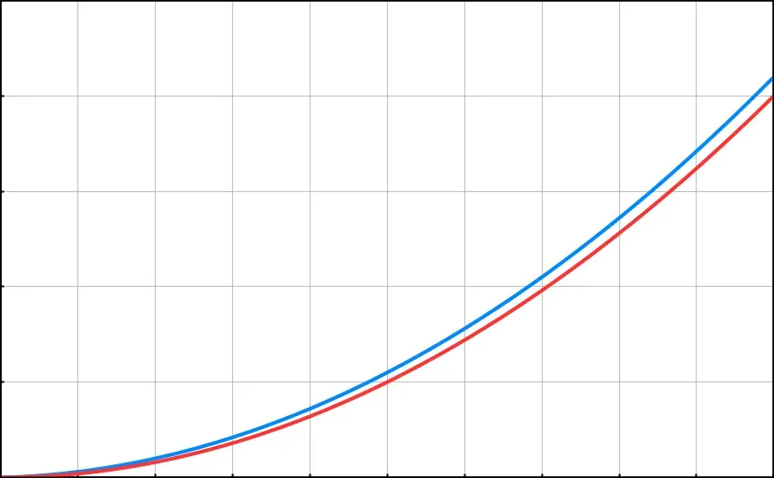
On the LEFT — Blue: (N² + N) · Red: O(N²). On the RIGHT — Blue: O(N³ + N² + N) · Red: O(N³ + N²) · Green: O(N³)
There are times where we need more precision, but in many situations it is sufficient to reduce expressions to the element that has the biggest impact on the algorithm as it scales.
With this and the rule about multiples, it is mostly expected that you would shorten an expression such as O(2N³ + 5N² + 4N + 7) to O(N³).
Logarithms
In order to understand the next section, we need to know what a logarithm is.
If you already know about logarithms, feel free to skip over to the next part.
For everyone else, logarithms are a different way of thinking about powers or exponents.
Take this statement: 2⁶ = 64
We can also express this as: log₂(64) = 6
In other words: Log base 2 of 64 equals 6.
The relationship between the number 2, 6 and 64 is the same in both equations. In a sense, we’re simply freeing up the 6 so we can perform other equations on it.
Logarithms are useful for a number of reasons, but here’s a very simple example. Say we didn’t know what the number x was: 2ˣ = 512
We can re-write the equation using logarithms to get: x = log₂(512)
Type that into a calculator, and we’ll get the answer 9. And, true enough, 2⁹ does equal 512.
If that makes sense, great. You’re ready to move on to the next example.
If you need to spend a little more time trying to understand logarithms, I recommend Khan Academy’s Introduction to Logarithms.
O(logN) — Binary Search
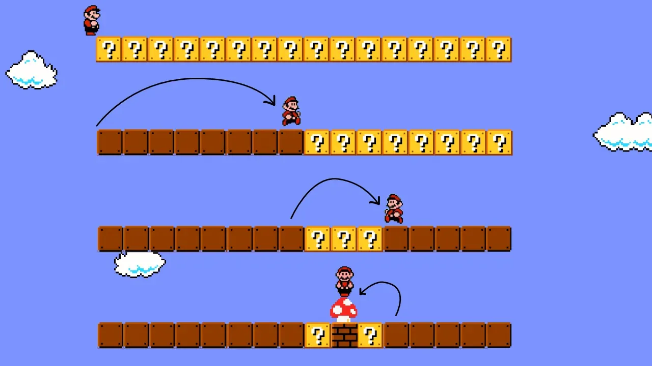
Image Credit: TopCoder
We need to understand the basics of logarithms because one of the most common and fastest search algorithms, the so-called “Binary Search” , has an efficiency of O(logN).
For most search requirements, Binary Search is the most efficient method possible.
A technical note: Technically, it’s O(log₂(N) + 1). In Computer Science we tend to assume the base is 2, so we can simply write O(logN), rather than O(log₂(N)). As for the +1, the minimum output cannot be zero, and the +1 accounts for this. However, as the O(logN) scales, the +1 becomes so small as to be irrelevant, and so we can safely ignore it.
First, I’ll explain what a Binary Search is, and then we can see how it is relevant to logarithms.
Let’s start with an array of numbers, from 1 to 15. For now, we’ll assume their already sorted from the smallest to the biggest.
let array = [1, 2, 3, 4, 5, 6, 7, 8, 9, 10, 11, 12, 13, 14, 15]
Now let’s say we want the computer to find the number 11.
A brute-force method to achieve this would have an efficiency of O(N), and might look something like this:
function findEleven(array) {
  for (let i = 0; i < array.length; i++) {
    if (array[i] === 11) {
      return i;
    }
  }
}
But we can do better! Here are the steps that the Binary Search method would take:
Stage
- The Binary Search method involves finding the mid-point of the array, which in this case is the number 8.
- 11 is higher than 8. That means we can cut the array in half, ignoring the numbers 1–7 and create a second array with the numbers 9–15.
Stage
- Let’s find the mid-point of our new array: that gives us the number 12.
- 11 is lower than 12. So we can cut our second array in half, ignoring 13–15, and create a third array with the numbers 9–11.
Stage
- Finally, we’ll cut the third array in half, giving us the number 10.
- 11 is higher than 10, and — as it happens — only one number is higher than 10: we’ve found it!
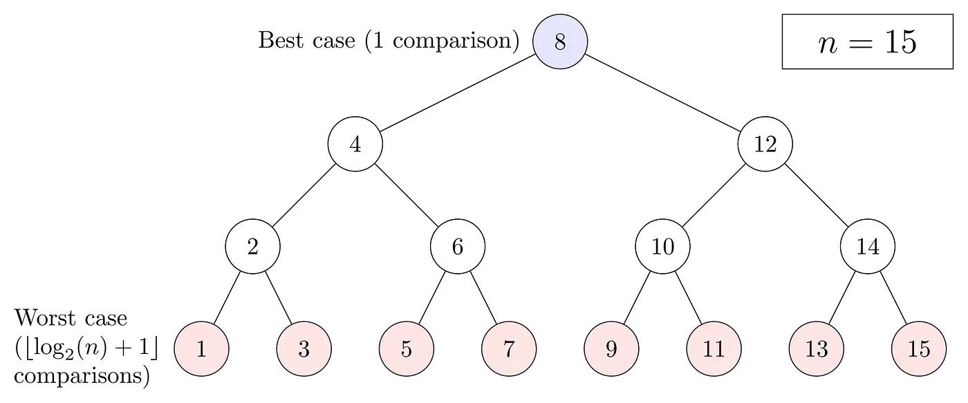
Image Credit: Wikipedia
For an array of this size, the maximum number of steps to the solution is 3. Compare that with the O(N) function. The maximum number steps it could take is 15.
If you double the data going into the Binary Search function, you get only 1 more step. But if you double the data going into the O(N) function, you get a potential 15 more steps!
Binary Search and Logarithms
This example makes clear how Binary Search is a much more efficient method, especially at scale.
But what has this to do with logarithms? It happens that, as more data is processed by a Binary Search function, the amount of processing time increases by a factor of logN.
Every time you double the data-set, an algorithm with performance O(logN) only has to add in 1 more step. The purple line below shows just how much more efficient logN can be than the other function types we have looked at so far.
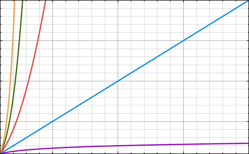
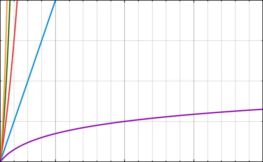
O(log(N)) is represented in purple. The image on the right is a zoomed-in (smaller scale) version of the image on the left.
Binary Search in JavaScript
Here’s what Binary Search might look like in JavaScript.
We’ll define a function that takes two parameters: an array of numbers (which must be sorted), and a search-value that we’re looking for.
function binarySearch(array, searchValue) {
  // Define start, end and pivot (middle)
  let start = 0;
  let end = array.length - 1;
  let pivot = Math.floor((start + end) / 2);

  // As long as the pivot is not our searchValue and the array is greater than 1, define a new start or end
  while (array[pivot] !== searchValue && start < end) {
    if (searchValue < array[pivot]) {
      end = pivot - 1;
    } else {
      start = pivot + 1;
    }

    // Every time, calculate a new pivot value
    pivot = Math.floor((start + end) / 2);
  }
  // If the current pivot is out search value, return it's index. Otherwise, return false.
  return array[pivot] === searchValue ? pivot : false;
}
O(NlogN) — Quicksort
For the final part of this article, we’ll look at one of the most efficient ways to sort through data — the Quicksort.
There are several different sorting algorithms with a performance of O(NlogN), including Merge sort, Heapsort, and Quicksort. But Quicksort tends to have the highest performance, so we’ll focus on it.
The main difference between sorting algorithms like these and Binary Search, described above, is that every time the sort algorithms pivot, they must go through the entire data set, finding out whether each value is higher or lower than the pivot value.
This process accounts for the appearance of the multiple N in O(NlogN) and this is what makes Quicksort (below, in cyan) slower than Binary Search (below, in purple).
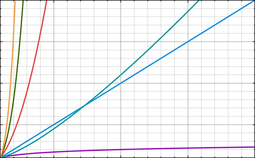
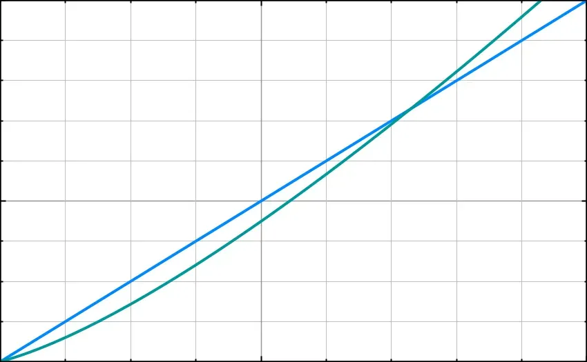
The cyan line represents O(Nlog(N)). Notice that, after a certain point, it becomes less efficient than O(N), represented in blue.
This is how a quicksort works:
Step 1
- Pick an element to be the pivot. In practice, this is usually the first or final element in the array.
Step 2
- Go through the array, comparing every value to the pivot.
- Values less than the pivot should be moved before it, while values greater than the pivot should come after it. This is called the partition operation.
- You are left with two sub-arrays: one with numbers greater than the pivot value; the other with numbers less than it.
Step 3
- Recursively apply steps 1 and 2 to each sub-array and repeat, until you can create no further sub-arrays.
- At that point, the sub-arrays are joined back into a single array.
The following image shows an example in practice, starting with the value 4 as our pivot:
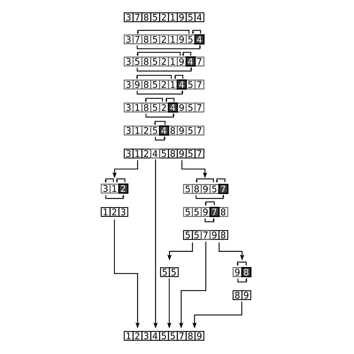
Image Credit: Wikipedia
Quicksort in JavaScript
function quicksort(array) {
  // If a sub-array has only 1 value, the array is sorted and can be returned
  if (array.length <= 1) {
    return array;
  }

  // Define pivot, and create empty "left" and "right" sub-arrays
  let pivot = array[0];
  let left = [];
  let right = [];

  // Go through the array, comparing values to the pivot, and sorting them into the "left" and "right" sub-arrays
  for (let i = 1; i < array.length; i++) {
    array[i] < pivot ? left.push(array[i]) : right.push(array[i]);
  }

  // Repeat using recursion
  return quicksort(left).concat(pivot, quicksort(right));
}
Final Word: Time and Space Complexity
In this article, we have focused solely on the time complexity of an algorithm. Time complexity is the amount of time taken by an algorithm to run relative to the length of the input.
We can also measure the efficiency of algorithms in terms of space complexity. This is the amount of space or memory used by an algorithm relative to the length of the input.
Both can be described using Big O Notation, and space complexity is bounded by time complexity. In other words, space and time complexity must be equal, or space complexity must be less.
The ins and outs of space complexity are beyond the remit of this article, but I hope the following quick example clarifies the difference.
Space Complexity in Bubble Sort, Binary Search and Quicksort
Above, we determined that the Bubble Sort has a time complexity of O(N²). But what about memory? When we sorted our example array, did we need to use any additional memory space?
We only had to define a single new variable, tmp. In fact, no matter the size of the input, we would still only need the one tmp variable. So that means the space complexity of the algorithm is just O(1).
Binary Search also has a space complexity of O(1), because the number of new variables created does not change relative to the size of the input.
For our final algorithm example, Quicksort, the space complexity depends on the implementation, since new arrays are created in the process. In our implementation, space complexity is O(logN).
If you’d like a slightly more detailed discussion of space complexity, that’s still beginner-friendly, I recommend this article.
Conclusion
At this point, we have covered most important cases of Big O Notation, and we’ve seen how they apply to three common algorithms for sorting and searching through data: the Bubble Sort, Binary Search, and Quicksort algorithms.
Equipped with this knowledge, you should be able to describe the performance of 90% of the algorithms you write using Big O Notation.
Of course, this topic can go deeper still. O(N) notation can, after all, describe an infinite number of patterns, and I’ve included a few links below to whet your appetite.
I Want To Know More
If you’re interested in learning more, there is — for example — a class of highly inefficient algorithms with a performance that decreases at a factorial rate of growth: one brute-force method for solving the Travelling Salesman Problem involves an algorithm of O(N!), while the so-called Bogosort, that has a performance of O(logN!).
There is also a class of algorithm that uses N as a power. For example, an algorithm of O(2ᴺ) may be used to solve the famous Tower’s of Hanoi puzzle.
Lastly, Big O Notation is just one of several types of notation used to measure algorithm’s performance. Technically, speaking, it measures the asymptotic upper bound. There’s also Big Omega Notation, which is written Ω(N), and which measures the asymptotic lower bound. And there’s Big Theta Notation, which is written Θ(N), and which measures the asymptotic tight bound. If you’re interested in learning more about these, this Medium article goes into greater detail.
Related articles
You might also enjoy...

Switching to a New Data Structure with Zero Downtime
A Practical Guide to Schema Migrations using TypeScript and MongoDB
7 min read

How to Automate Merge Requests with Node.js and Jira
A quick guide to speed up your MR or PR workflow with a simple Node.js script
7 min read

Automate Your Release Notes with AI
How to save time every week using GitLab, OpenAI, and Node.js
11 min read